Thicket and Extra-P: Thicket Tutorial

Thicket is a python-based toolkit for Exploratory Data Analysis (EDA) of parallel performance data that enables performance optimization and understanding of applications’ performance on supercomputers. It bridges the performance tool gap between being able to consider only a single instance of a simulation run (e.g., single platform, single measurement tool, or single scale) and finding actionable insights in multi-dimensional, multi-scale, multi-architecture, and multi-tool performance datasets.

This notebook provides an example for using Thicket’s modeling feature. The modeling capability relies on Extra-P - a tool for empirical performance modeling. It can perform N-parameter modeling with up to 3 parameters (N <= 3). The models follow a so-called Performance Model Normal Form (PMNF) that expresses models as a summation of polynomial and logarithmic terms. One of the biggest advantages of this modeling method is that the produced models are human-readable and easily understandable.

NOTE: An interactive version of this notebook is available in the Binder environment.

1. Import Necessary Packages

To explore the capabilities of thicket with Extra-P, we begin by importing necessary packages.

[1]:

import sys

import matplotlib.pyplot as plt
import pandas as pd
from IPython.display import display
from IPython.display import HTML

import thicket as th
from thicket.model_extrap import Modeling

display(HTML("<style>.container { width:80% !important; }</style>"))

2. Define Dataset Paths and Names

In this example, we use an MPI scaling study, profiled with Caliper, that has metadata about the runs. The data is also already aggregated, which means we can provide the data to Extra-P as-is.

[2]:

data = "../data/mpi_scaling_cali"
t_ens = th.Thicket.from_caliperreader(data)

/opt/conda/lib/python3.9/site-packages/thicket/ensemble.py:319: FutureWarning: A value is trying to be set on a copy of a DataFrame or Series through chained assignment using an inplace method.
The behavior will change in pandas 3.0. This inplace method will never work because the intermediate object on which we are setting values always behaves as a copy.

For example, when doing 'df[col].method(value, inplace=True)', try using 'df.method({col: value}, inplace=True)' or df[col] = df[col].method(value) instead, to perform the operation inplace on the original object.


  perfdata[col].replace({fill_value: None}, inplace=True)

Specifically, the metadata table for this set of profiles contains a jobsize column, which provides the amount of cores used for each profile.

[3]:

t_ens.metadata["jobsize"]

[3]:

profile
27654391       64
91138395      343
368928273      27
964810492     216
1734033023    125
Name: jobsize, dtype: int64

3. More Information on a Function

You can use the help() method within Python to see the information for a given object. You can do this by typing help(object). This will allow you to see the arguments for the function, and what will be returned. An example is below.

[4]:

help(Modeling)

Help on class Modeling in module thicket.model_extrap:

class Modeling(builtins.object)
 |  Modeling(tht, param_name, params=None, chosen_metrics=None)
 |
 |  Produce models for all the metrics across the given graphframes.
 |
 |  Methods defined here:
 |
 |  __init__(self, tht, param_name, params=None, chosen_metrics=None)
 |      Create a new model object.
 |
 |      Adds a model column for each metric for each common frame across all the
 |      graphframes.
 |
 |      The given list of params contains the parameters to build the models.  For
 |      example, MPI ranks, input sizes, and so on.
 |
 |      Arguments:
 |          tht (Thicket): thicket object
 |          param_name (str): arbitrary if 'params' is being provided, otherwise name of
 |              the metadata column from which 'params' will be extracted
 |          params (list): parameters list, domain for the model
 |          chosen_metrics (list): metrics to be evaluated in the model, range for the
 |              model
 |
 |  componentize_statsframe(self, columns=None)
 |      Componentize multiple Extra-P modeling objects in the aggregated statistics
 |      table
 |
 |      Arguments:
 |          column (list): list of column names in the aggregated statistics table to
 |              componentize. Values must be of type 'thicket.model_extrap.ModelWrapper'.
 |
 |  produce_models(self, agg_func=<function mean at 0xffff59d001f0>, add_stats=True)
 |      Produces an Extra-P model. Models are generated by calling Extra-P's
 |          ModelGenerator.
 |
 |      Arguments:
 |          agg_func (function): aggregation function to apply to multi-dimensional
 |              measurement values. Extra-P v4.0.4 applies mean by default so that is
 |              set here for clarity.
 |          add_stats (bool): Option to add hypothesis function statistics to the
 |              aggregated statistics table
 |
 |  to_html(self, RSS=False)
 |
 |  ----------------------------------------------------------------------
 |  Data descriptors defined here:
 |
 |  __dict__
 |      dictionary for instance variables (if defined)
 |
 |  __weakref__
 |      list of weak references to the object (if defined)

3. Create Models

First, we construct the Modeling object by passing all the relevant data to it. We provide jobsize as the param_name argument so the model will grab this column from the metadata table to use as our parameter. We also sub-select some metrics, since this dataset has a lot of metrics (otherwise the modeling will take a long time to do all metrics).

Then, we call produce_models on that object (it’s unnecessary to provide an aggregation function since the data is already aggregated.).

NOTE: For this example, you can view all the metric columns by adding a new cell and running: t_ens.performance_cols.

[5]:

mdl = Modeling(
    t_ens,
    "jobsize",
    chosen_metrics=[
        "Total time",
    ],
)

mdl.produce_models()

4. Models Dataframe

Model hypothesis functions are stored in thicket’s aggregated statistics table.

[6]:

t_ens.statsframe.dataframe

[6]:

	name	Total time_extrap-model	Total time_RSS_extrap-model	Total time_rRSS_extrap-model	Total time_SMAPE_extrap-model	Total time_AR2_extrap-model	Total time_RE_extrap-model
node
{'name': 'MPI_Allreduce', 'type': 'function'}	MPI_Allreduce	-0.0024835738301864883 + 4.6723137107329955e-0...	2.373695e-02	33.638540	71.854711	0.982806	1.569021
{'name': 'MPI_Bcast', 'type': 'function'}	MPI_Bcast	0.005594622766668683 + 1.1211777143604538e-05 ...	5.234884e-03	0.592849	18.775441	0.994136	0.222561
{'name': 'MPI_Comm_dup', 'type': 'function'}	MPI_Comm_dup	0.20714199930961863 + 0.0003794872132338881 * ...	1.468475e+01	1.458439	50.350316	0.324860	0.467371
{'name': 'MPI_Comm_free', 'type': 'function'}	MPI_Comm_free	2.9748964461513302e-05 + 2.9632810629043044e-0...	4.012398e-08	0.026386	5.697692	0.995381	0.054844
{'name': 'MPI_Comm_split', 'type': 'function'}	MPI_Comm_split	0.0340992099469718 + 4.861767349462252e-07 * p...	4.094649e+00	1.584798	40.927787	0.904711	0.445655
{'name': 'MPI_Gather', 'type': 'function'}	MPI_Gather	1.1110717100841163e-05 + 1.875931772029739e-09...	1.805567e-07	2.319450	37.410684	0.857675	0.515782
{'name': 'MPI_Initialized', 'type': 'function'}	MPI_Initialized	-1.2157511991333312e-06 + 4.473650007736346e-0...	2.079887e-09	0.016595	4.528570	0.997857	0.046511
{'name': 'main', 'type': 'function'}	main	5.3345854025532375 + 50.4472239870803 * p^(1)	1.428021e+07	0.132731	15.651588	0.886893	0.157082
{'name': 'MPI_Barrier', 'type': 'function'}	MPI_Barrier	-3.8613044063814517 + 0.7228867130047671 * log...	7.133681e+00	80964.639853	127.158285	-0.330302	65.337903
{'name': 'MPI_Irecv', 'type': 'function'}	MPI_Irecv	0.00016930423157778974 + 5.344486361848511e-05...	5.902043e-04	0.048232	8.436975	0.985537	0.084786
{'name': 'MPI_Isend', 'type': 'function'}	MPI_Isend	-0.7378766027055433 + 0.011372374310428854 * p...	5.386096e-01	5023.400772	80.306304	0.937724	19.620193
{'name': 'MPI_Reduce', 'type': 'function'}	MPI_Reduce	0.008950513364525873 + 2.1551606902927176e-05 ...	1.756609e-03	32.371981	49.251316	0.436922	1.295318
{'name': 'MPI_Wait', 'type': 'function'}	MPI_Wait	-0.08273770855385487 + 0.0008985035981343798 *...	2.613648e-01	15.106425	50.478159	0.567859	1.000543
{'name': 'MPI_Waitall', 'type': 'function'}	MPI_Waitall	0.0118324	1.275860e-03	282.767881	109.810235	1.000000	3.622031
{'name': 'lulesh.cycle', 'type': 'function'}	lulesh.cycle	6.361023656690073 + 50.40069659189232 * p^(1)	1.431665e+07	0.133362	15.688203	0.886407	0.157454
{'name': 'LagrangeLeapFrog', 'type': 'function'}	LagrangeLeapFrog	-588.7139217783075 + 118.0201880558251 * p^(4/5)	3.026414e+06	0.040647	7.619168	0.947871	0.076241
{'name': 'CalcTimeConstraintsForElems', 'type': 'function'}	CalcTimeConstraintsForElems	0.2912128378771341 + 0.15464468104595394 * p^(1)	6.423611e-01	0.010278	2.671244	0.999446	0.027639
{'name': 'LagrangeElements', 'type': 'function'}	LagrangeElements	55.8023570683435 + 12.21983926020424 * p^(1)	2.180612e+05	0.041861	8.942728	0.970060	0.089881
{'name': 'ApplyMaterialPropertiesForElems', 'type': 'function'}	ApplyMaterialPropertiesForElems	6.909192329599326 + 3.812718071421941 * p^(1)	1.344775e+03	0.001975	1.640254	0.998092	0.016486
{'name': 'EvalEOSForElems', 'type': 'function'}	EvalEOSForElems	7.437812732121266 + 3.719775901083089 * p^(1)	1.057620e+03	0.001701	1.524714	0.998424	0.015326
{'name': 'CalcEnergyForElems', 'type': 'function'}	CalcEnergyForElems	7.3616219620609575 + 2.352394804115736 * p^(1)	1.943577e+02	0.001304	1.490833	0.999275	0.015001
{'name': 'CalcLagrangeElements', 'type': 'function'}	CalcLagrangeElements	-3.807204897434417 + 1.5032184055481064 * p^(3...	7.778453e+02	0.002324	1.859640	0.998118	0.018461
{'name': 'CalcKinematicsForElems', 'type': 'function'}	CalcKinematicsForElems	-3.191063749981387 + 1.440739634475724 * p^(3/...	9.575080e+02	0.002845	1.935065	0.997478	0.019204
{'name': 'CalcQForElems', 'type': 'function'}	CalcQForElems	6.979231420889168 + 2.799033804303159 * p^(3/4...	3.048464e+05	0.191824	17.597453	0.795277	0.175135
{'name': 'CalcMonotonicQForElems', 'type': 'function'}	CalcMonotonicQForElems	-4.021092516288899 + 0.49595942520127567 * p^(...	1.628638e+02	0.014441	4.535001	0.996383	0.044701
{'name': 'MPI_Irecv', 'type': 'function'}	MPI_Irecv	0.020640239201916117 + 0.0009474689031858098 *...	1.147505e-02	0.003239	2.299890	0.997552	0.023065
{'name': 'MPI_Isend', 'type': 'function'}	MPI_Isend	-0.10548527169972247 + 0.004772194045454103 * ...	1.151804e+00	0.009142	3.781670	0.990329	0.038011
{'name': 'MPI_Wait', 'type': 'function'}	MPI_Wait	58.43177001577187 + 0.10805277471434777 * p^(3...	2.687218e+05	2.301295	46.138279	-0.265790	0.504422
{'name': 'MPI_Waitall', 'type': 'function'}	MPI_Waitall	-28.32003046236924 + 0.5649498323219662 * p^(1...	1.854066e+03	7.732766	40.064332	0.819884	0.720597
{'name': 'LagrangeNodal', 'type': 'function'}	LagrangeNodal	-501.7214996437166 + 103.6028442396303 * p^(3/4)	1.307338e+06	0.052532	9.539895	0.945355	0.096236
{'name': 'CalcForceForNodes', 'type': 'function'}	CalcForceForNodes	-483.43658919501837 + 94.44404618163018 * p^(3/4)	7.615735e+05	0.028787	6.373836	0.961502	0.063767
{'name': 'CalcVolumeForceForElems', 'type': 'function'}	CalcVolumeForceForElems	-8.924824714807004 + 18.087142774934236 * p^(1)	4.205287e+04	0.007481	3.251360	0.997349	0.033025
{'name': 'CalcHourglassControlForElems', 'type': 'function'}	CalcHourglassControlForElems	-18.407641701934274 + 15.299434861302805 * p^(1)	3.933893e+04	0.005348	3.043918	0.996535	0.030703
{'name': 'CalcFBHourglassForceForElems', 'type': 'function'}	CalcFBHourglassForceForElems	-3.454147978296185 + 1.9523476557370125 * p^(3...	4.555233e+02	0.007429	2.856552	0.999346	0.028786
{'name': 'IntegrateStressForElems', 'type': 'function'}	IntegrateStressForElems	-3.2210357806507735 + 1.3155188131276156 * p^(...	9.669293e+02	0.003183	2.237380	0.996946	0.022230
{'name': 'MPI_Irecv', 'type': 'function'}	MPI_Irecv	0.07139784821037228 + 0.0012913170911470285 * ...	1.217607e-02	0.038615	4.834306	0.999487	0.051334
{'name': 'MPI_Isend', 'type': 'function'}	MPI_Isend	-0.13477165012239584 + 0.006980575896793848 * ...	4.308979e-01	0.005076	2.843889	0.998306	0.028019
{'name': 'MPI_Wait', 'type': 'function'}	MPI_Wait	200.4196336	6.491636e+04	23.569468	57.976850	1.000000	0.401049
{'name': 'MPI_Waitall', 'type': 'function'}	MPI_Waitall	-60.47462228639048 + 15.850591840236687 * p^(2/3)	2.200269e+05	124572.019480	70.449504	0.197527	70.913096
{'name': 'MPI_Irecv', 'type': 'function'}	MPI_Irecv	-0.05528188247031427 + 0.005354748856582524 * ...	7.789738e-01	0.144243	13.336394	0.856270	0.133853
{'name': 'MPI_Isend', 'type': 'function'}	MPI_Isend	-0.03796477449325472 + 0.00852182055673094 * p...	9.730921e+00	0.178043	17.445265	0.867448	0.182547
{'name': 'MPI_Wait', 'type': 'function'}	MPI_Wait	-98.98907610355376 + 23.56658785930815 * log2(...	9.984181e+03	93.165856	73.120318	-0.360185	2.393805
{'name': 'MPI_Waitall', 'type': 'function'}	MPI_Waitall	-90.56809038671453 + 5.542383651985729 * log2(...	6.315946e+04	2.822066	37.003734	-0.214628	0.477486
{'name': 'TimeIncrement', 'type': 'function'}	TimeIncrement	108.79336164114378 + 0.41659851800619824 * p^(...	5.231852e+06	0.681284	34.858860	0.614904	0.339668
{'name': 'MPI_Allreduce', 'type': 'function'}	MPI_Allreduce	108.66456642370454 + 0.41649782186503276 * p^(...	5.232565e+06	0.681661	34.862073	0.614677	0.339689

5. Show the Models Dataframe with Embedded Plots

(For every node, sub-selected metric combination)

[7]:

with pd.option_context("display.max_colwidth", 1):
    display(HTML(mdl.to_html()))

	Total time_extrap-model
node
{'name': 'MPI_Allreduce', 'type': 'function'}
{'name': 'MPI_Bcast', 'type': 'function'}
{'name': 'MPI_Comm_dup', 'type': 'function'}
{'name': 'MPI_Comm_free', 'type': 'function'}
{'name': 'MPI_Comm_split', 'type': 'function'}
{'name': 'MPI_Gather', 'type': 'function'}
{'name': 'MPI_Initialized', 'type': 'function'}
{'name': 'main', 'type': 'function'}
{'name': 'MPI_Barrier', 'type': 'function'}
{'name': 'MPI_Irecv', 'type': 'function'}
{'name': 'MPI_Isend', 'type': 'function'}
{'name': 'MPI_Reduce', 'type': 'function'}
{'name': 'MPI_Wait', 'type': 'function'}
{'name': 'MPI_Waitall', 'type': 'function'}
{'name': 'lulesh.cycle', 'type': 'function'}
{'name': 'LagrangeLeapFrog', 'type': 'function'}
{'name': 'CalcTimeConstraintsForElems', 'type': 'function'}
{'name': 'LagrangeElements', 'type': 'function'}
{'name': 'ApplyMaterialPropertiesForElems', 'type': 'function'}
{'name': 'EvalEOSForElems', 'type': 'function'}
{'name': 'CalcEnergyForElems', 'type': 'function'}
{'name': 'CalcLagrangeElements', 'type': 'function'}
{'name': 'CalcKinematicsForElems', 'type': 'function'}
{'name': 'CalcQForElems', 'type': 'function'}
{'name': 'CalcMonotonicQForElems', 'type': 'function'}
{'name': 'MPI_Irecv', 'type': 'function'}
{'name': 'MPI_Isend', 'type': 'function'}
{'name': 'MPI_Wait', 'type': 'function'}
{'name': 'MPI_Waitall', 'type': 'function'}
{'name': 'LagrangeNodal', 'type': 'function'}
{'name': 'CalcForceForNodes', 'type': 'function'}
{'name': 'CalcVolumeForceForElems', 'type': 'function'}
{'name': 'CalcHourglassControlForElems', 'type': 'function'}
{'name': 'CalcFBHourglassForceForElems', 'type': 'function'}
{'name': 'IntegrateStressForElems', 'type': 'function'}
{'name': 'MPI_Irecv', 'type': 'function'}
{'name': 'MPI_Isend', 'type': 'function'}
{'name': 'MPI_Wait', 'type': 'function'}
{'name': 'MPI_Waitall', 'type': 'function'}
{'name': 'MPI_Irecv', 'type': 'function'}
{'name': 'MPI_Isend', 'type': 'function'}
{'name': 'MPI_Wait', 'type': 'function'}
{'name': 'MPI_Waitall', 'type': 'function'}
{'name': 'TimeIncrement', 'type': 'function'}
{'name': 'MPI_Allreduce', 'type': 'function'}

6. Query Specific Model

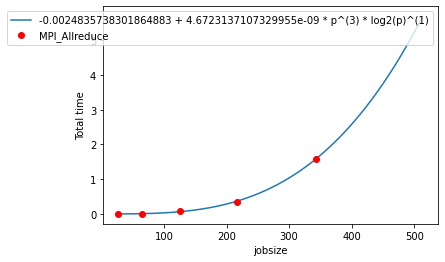
The 1st node {"name": "MPI_Allreduce", "type": "function"}, has an interesting graph so we want to retrieve its model. This can be achieved by indexing into the aggregated statistics table for our chosen node for the metric Total time_extrap-model.

[8]:

model_obj = t_ens.statsframe.dataframe.at[t_ens.statsframe.dataframe.index[0], "Total time_extrap-model"]

7. Operations on a model

We can evaluate the model at a value like a function.

[9]:

model_obj.eval(600)

[9]:

9.311422624087944

Displaying the model:

It returns a figure and an axis objects. The axis object can be used to adjust the plot, i.e., change labels. The display() function requires an input for RSS (bool), that determines whether to display Extra-P RSS on the plot.

[10]:

plt.clf()
fig, ax = model_obj.display(RSS=False)
plt.show()

<Figure size 432x288 with 0 Axes>

_images/extrap-with-metadata-aggregated_19_1.png